


 Inglés (pdf)
 Articulo en XML
 Referencias del artículo

 Permalink
1. Introduction
Worldwide, irrigated agricultural production accounts for over 70% of water withdrawals1. In Uruguay, the percentage of water used for this sector is even higher. According to De León & Delgado2, 86% of the volume of water used in Uruguay is destined for agricultural irrigation, which coincides with data from Hill3, reporting 84% of the extracted water used for the same purpose, and from DINAGUA4, which reports 80% of the use of extracted water for crop irrigation.
Between the 1970s and 2000s, the irrigated area in Uruguay experienced a significant increase, quadrupling its area from 52,000 to 218,000 irrigated hectares, according to Hill3, with rice being the agricultural item that has determined the evolution of the country's irrigated area. However, despite this increase, only 15% of the country's total cultivated area is currently irrigated. On the other hand, since 2010-11 the rice-planting area has been decreasing, leading to the underutilization of significant volumes of reservoir water that is available and idle. Intensive livestock production with planted and irrigated pastures in direct grazing could be an immediate alternative for these regions of the country5.
Regarding pasture irrigation, information in Uruguay is scarce, but according to 2011 data, only 1.2% of grazing crops were irrigated, as reported by DIEA6.
Between 80 and 85% of the world's irrigated area is carried out using surface irrigation 7)(8) . Despite the economic advantages of surface irrigation, such as lower investment and operational costs compared to pressurized irrigation7, these advantages are counterbalanced by the need for precise systematization, coupled with the unsuitability of this irrigation method for light-textured soils9.
There is no such thing as an optimal irrigation method; rather, the appropriateness of a method depends on the specific situation10. Among the different types of surface irrigation, border irrigation is the one that is best adapted to forage crops. García Petillo10 suggests that low application efficiency (AE) or distribution uniformity (DU) in surface irrigation cannot be attributed to the method itself if the irrigation system has not been properly designed or operated. High-slope topography and low infiltration rates represent additional challenges for adapting international guidelines 11) in the management of border irrigation. Faced with this situation, the Hydrology, Irrigation and Drainage Unit of the Agronomy College (Udelar) initiated, in 2012, a line of research on border irrigation in pastures, aiming to optimize irrigation management from design to management decision-making.
Various national investigations have reported mixed results regarding application efficiency and distribution uniformity in surface irrigation systems, ranging from high to low levels. According to García Petillo and others11, the first study of the Hydrology, Irrigation and Drainage Unit in this type of surface irrigation did not achieve acceptable levels of distribution uniformity (DU) or application efficiency (AE), attributable to the presence of transverse slope in the border. In this case, AE values of 13% and DU of 62% were recorded. In response to this problem, the following study carried out by Puppo and others12 prioritized the systematization of the border irrigation test, defining the direction of the border in the direction of the maximum slope, minimizing the transverse slope, reaching DU values above 90%, with AE in a medium range between 40 and 50%.
In the research carried out by Corcoll & Malvasio13, the average AE and DU for three irrigation sheets applied were 91.2% and 91.6%, respectively. In accordance with these studies, Bourdin and others 14) obtained AE values above 75%, coinciding with the application efficiency results obtained by Ribas & García15. This last study was conducted on two different types of soils, resulting in AE values above 75%. These observations suggest that the optimization of efficiency in surface irrigation is closely linked to proper farm systematization.
WinSRFR is a hydraulic simulation model of surface irrigation developed by the USDA-Agricultural Research Service that allows the analysis of surface irrigation performance by evaluating performance parameters, estimating water infiltration, and simulating new irrigation scenarios16. In the study carried out by Puppo and others12, WinSRFR accurately predicted the volume of infiltrated and runoff water, and Corcoll & Malvasio13 concluded that the WinSRFR simulation model exhibited a good correlation between observed field data and those simulated by the model, in terms of AE.
The WinSRFR model has been widely used in various studies, either for calibration purposes or simply for the analysis of field results, including the studies by Puppo and others12, Corcoll & Malvasio13, Bourdin Medici and others14, and Ribas & García15. Bautista and others16 performed a sensitivity analysis of the model to variations in the infiltration family and Manning’s roughness coefficient (n), under conditions of fixed irrigation dimensions and time. Their study indicates that the model responds to variations in these factors, although in some cases the effect is minimal. It should be noted that this study did not consider variations in slope, conducting all simulations with a fixed slope. While international literature recommends surface irrigation17 for low slopes, border irrigation practices are common in Uruguay on pastures with slopes of 3% or more. Therefore, studying the model's sensitivity to variations in this parameter is important.
In this context, our study aimed to continue adjusting border irrigation technology for the soil and topographic conditions of southern Uruguay, and to validate the performance of the WinSRFR model in border irrigation with pastures. Additionally, technical recommendations for border irrigation are proposed for soil and topographic conditions different from those evaluated in this study, aiming to serve as a tool for the design and management of border irrigation in pastures.
2. Material and methods
2.1 Test site and characterization
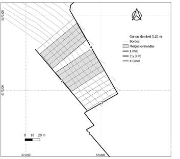
The study was conducted at the Southern Regional Center of the Agronomy College in Progreso, Canelones (34º36'26.38'' S, 56º13'03.36'' W). In February 2016, a topographic survey was carried out with contour lines at vertical intervals of 0.2 m. Subsequently, the irrigation area was systematized, orienting the plots in the direction of maximum slope to minimize transverse slope.
The soil corresponds to Argiudolls and Hapluderts, according to the USDA classification18. It is classified as Typic Eutric Brunosol, black or very dark brown, with loamy silty clay texture, high fertility and moderately well-drained, and with slopes ranging from 1 to 4%. It belongs to the Tala Rodriguez Soil Unit of the 1:1 million chart; representative of the Coneat soil group: 10.8a.
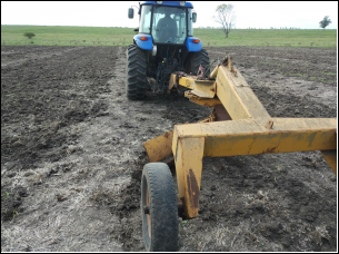
In April 2020, surface roughness was removed and the edges of the borders were reshaped using a tail shovel. Figure 1 shows the borders and the machinery forming the edges.
A total of 14 borders were traced, with a longitudinal slope of between 1.5 and 3%, widths of 5.5 to 6.3 m and lengths of 50-65 m (Table 1).
Table 1: Dimensions of each border
| Border | 1 | 2 | 3 | 4 | 5 | 6 | 7 | 8 | 9 | 10 | 11 | 12 | 13 | 14 |
| Length (m) | 65 | 64 | 63 | 63 | 62 | 58 | 57 | 56 | 55 | 55 | 53 | 52 | 51 | 50 |
| Width (m) | 5.8 | 5.9 | 5.8 | 5.5 | 5.9 | 5.5 | 5.8 | 5.5 | 5.9 | 5.9 | 6.0 | 6.3 | 6.1 | 5.9 |
| Long. slope (%) | 2.9 | 2.8 | 2.9 | 2.8 | 2.7 | 2.3 | 2.6 | 2.7 | 2.7 | 2.7 | 2.5 | 2.1 | 2.3 | 1.5 |
Long. slope= longitudinal slope
From the total built, 9 borders were selected to carry out the test, choosing those with the greatest length and dimensions close to those used by Puppo and others12, for which the range of flow rates to evaluate had already been defined.
On May 29, 2020, a mixture of fescue, white clover, and lotus was sown. Irrigation water was diverted from the reservoir, initially using a polyethylene (PE) siphon with a nominal diameter (ND) of 110 mm. During the drought of 2021-22 and 2022-23, the water diversion from the reservoir to the area systematized for border irrigation had to be replaced by a motor pump to be able to pump from a lower level in the reservoir. Conduction to the borders was carried out with collapsible polyethylene sleeves of 10" and 250 microns (Figure 2). The water was adduced to each border by means of two adjustable 2" gates, spaced 3 m apart.
2.2 Soil water parameters
The field capacity (FC) of each horizon was determined using the methodology proposed by García Petillo and others19, while the permanent wilting point (PWP) was estimated by means of the regression developed by Silva and others20 based on the FC data on a dry weight basis. Bulk density by horizon measurement was performed using undisturbed samples.
Table 2: Soil hydraulic parameters
| Depth cm | FC % dw | PWP % dw | Db g cm-3 | AW mm 10 cm-1 | AW mm horiz-1 |
| 0-20 | 28.8% | 16.6% | 1.2 | 15 | 29 |
| 20-40 | 31.6% | 18.7% | 1.17 | 15 | 30 |
| Total | 59 |
FC % dw = field capacity on a dry weight basis; PWP % dw = permanent wilting point on a dry weight basis; Db = bulk density; AW = available water
Cumulative infiltration was measured using the double-ring infiltrometer technique. A curve was fitted using Kostyakov's equation, expressed as follows:
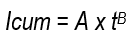
where Icum represents the cumulative infiltration as a function of time in millimeters, A and B are the coefficient and exponent of the potential equation, respectively, and t is the time of water entry into the soil in minutes.
Subsequently, based on the data from the irrigation assessments, the coefficient A of equation (1) was corrected by means of a volume balance, resulting in a new Amodif coefficient. This correction was carried out to enable the application of the WinSRFR 16)(21) simulation model, with the following ratio:
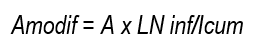
where Amodif = coefficient of the infiltration equation modified; A = coefficient of the infiltration equation with double-ring infiltrometer; LN inf = average infiltrated sheet calculated by volume balance in each evaluation; Icum = average infiltrated sheet calculated with the double-ring infiltrometer equation in each evaluation, determined by contact time.
The infiltration rate, in mm h-1, was obtained by deriving the cumulative infiltration as a function of time. Basic soil infiltration, Ib, was determined by the following formula 17)(22) :
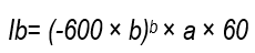
where Ib = the basic infiltration of the soil in mm h-1; A = the coefficient of the infiltration rate equation, and B = the exponent of the infiltration rate equation, from data expressed in mm and min. The Ib is determined in order to define which infiltration family23 the test soil is part of.
2.3 Flow rates and irrigation time evaluated
As a starting point for flow application, the optimized flow rates previously determined by Puppo and others12 were adopted, with a greater reduction in flow rate due to the high runoff volumes observed when using a high flow rate for the dimensions of the borders evaluated. The evaluated unit flow rates were as follows: Q1 = 0.2, Q2 = 0.33 and Q3 = 0.4 L s-1 m-1, with three repetitions each. The inflow rates were finally set for the width of the plots at 1.2, 2.0 and 2.4 L s-1, corresponding to Q1, Q2 and Q3, respectively.
Table 3 shows the characteristics of the borders used with each flow rate. The lengths varied between 55 and 64 m, the width of each border from 5.5 to 6.0, and the slope from 2.3 to 2.9%.
Table 3: Characteristics of the furrows used in each evaluation
| Variable | Q1 | Q2 | Q3 |
| Inflow rate (L s-1 m-1) | 0.20 | 0.33 | 0.40 |
| Length (m) | 55 - 63 | 55 - 63 | 57 - 64 |
| Width (m) | 5.5 - 6.0 | 5.5 - 5.9 | 5.8 - 5.9 |
| Slope (%) | 2.7 - 2.8 | 2.3 - 2.9 | 2.6 - 2.8 |
Soil moisture was monitored using an FDR (Frequency Domain Reflectometry, Delta-T Devices™, USA) probe before and after each evaluation. Eight access pipes were installed in 6 plots, and 3 pipes in 3 other plots to determine the volumetric moisture content. The probe was calibrated to measure at two depths, from 0 to 20 cm and from 20 to 40 cm (maximum depth reached by absorbing roots), using the gravimetric method of soil water measurement, according to Marano and others24.
Regarding the irrigation time (IT), upon finding that the flow rates optimized by Puppo and others12 did not match the expected time for their application, the WinSRFR Operational Analysis was used. This analysis allowed determining the irrigation time required to ensure the infiltration of the required sheet at the foot of the borders before each evaluation 16)(21) .
Before each evaluation, the net sheet required to restore soil moisture to FC at root depth (LN) was defined. For this purpose, the FDR probe was used to measure soil moisture before irrigation, and the required IT for each flow rate was calculated, as mentioned previously, using the results of the Operational Analysis module of the WinSRFR model. The inputs needed by this module are border dimensions, longitudinal slope, infiltration rate and Manning's roughness coefficient (n), where n used was 0.3.
2.4 Field determinations
In each evaluation, inflow and outflow hydrographs were generated for the three evaluated flow rates. To do this, WSC flowmeters were installed at the inlet of each border to measure the inflow, and a channel was designed at the foot of the borders where WSC flowmeters were located to measure the outflow. Two different sizes of flowmeters were used, adapted to the range of flow rates to measure. The selection of these flowmeters is based on their recommendation for measuring small flow rates25.
In order to construct the advance and recession curves for each flow rate, stakes were placed in the evaluated plots every 10 meters. The time of arrival and recession of water at each stake was recorded, thus defining the contact time.
2.5 Performance parameters
From pre- and post-irrigation moisture levels, inflow and outflow hydrographs, and advance and recession curves, various efficiency indicators or performance parameters were calculated, including Application Efficiency (AE), Distribution Uniformity (DU), Storage Efficiency (RE), Percolation Losses (Per), and Runoff (RO). AE was determined as the ratio of the infiltrated sheet at root depth (LN inf) to the gross sheet (LB).
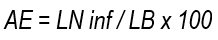
LN inf represents the sheet that was effectively infiltrated and stored at root depth, measured in millimeters, and was calculated according to García Petillo and others19 using the formula:
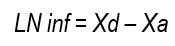
where Xa is the average water content in millimeters of all points before irrigation, determined with the FDR probe, and Xd is the average water content in millimeters of all points after irrigation, also measured with the FDR probe. On the other hand, LB, which corresponds to the total sheet applied in millimeters, was determined with the following formula:
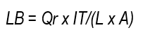
where Qr is the irrigation flow rate at L s-1; IT is the irrigation time in s; L is the length of the border in meters, and A is the width of the border in m.
DU was calculated as the ratio between the infiltrated sheet in the least irrigated quarter and the average infiltrated sheet in the entire plot, following the method of Walker & Skogerboe26. The average infiltrated sheet was calculated from the volume balance, defining the following formula:
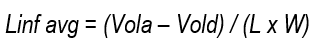
where Linf avg = average infiltrated sheet in the border, in mm; Vola = total volume applied in L; Vold = total volume drained in L; L = length of the border in m; W = width of the border in m.
Since the average infiltrated sheet is related to the contact time, the infiltrated sheet in the least irrigated quarter corresponded to the quarter of data taken in the plot with the shortest contact time (T recession - T advance), that is, the shortest time the water remains on the soil surface. To calculate this, the contact time of the least irrigated quarter was substituted into the cumulative infiltration equation (1) and the modified A coefficient (2) was used.
RE is the ratio between the net sheet stored (LN inf(5)) after irrigation, and the net sheet required (LN).

Runoff (RO) was defined with the following formulas:

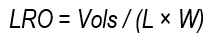
where LRO is the runoff sheet (in mm), calculated as the volume of water determined with flowmeters in the channel at the foot of the border relative to the area of the border; LB corresponds to the total sheet applied in millimeters; Vols is the total runoff volume in liters measured with a flowmeter at the foot of the borders; L the length of the border in meters, and W the width of the border in m.
Finally, percolation losses (Per) are defined as the difference between the above efficiencies:

2.6 Use of the WinSRFR program and its validation
For each evaluation and flow rate, the Simulation module in the WinSRFR program was used to replicate the field evaluations and observe how well the model predicts the results. The input data needed for this module are: LN, inflow hydrographs, border dimensions, longitudinal slope, infiltration rate and Manning's roughness coefficient (n), where the n used was 0.3.
A preliminary analysis was performed to compare the performance parameters obtained during the field evaluations with the parameters generated by the simulation module (observed values, average, minimum and maximum values). In this initial analysis, for each evaluation and flow rate, the Kostiakov equation (1) was used for the infiltration rate in the simulation module, with the Amodif obtained through volume balance (2). That is, each event was adjusted by volume balance. This last aspect is crucial in our study, given that each assessment was conducted under disparate soil moisture conditions. Therefore, the need to adjust the infiltration rate using volume balance becomes fundamental in every evaluation. From now on, this analysis methodology is referred to as Simulation with Amodif.
Considering that obtaining Amodif requires determining the runoff in the field to define the volume balance, and recognizing that this process can be challenging at the producer level, the option arises to compare performance parameters using the infiltration family, defined from the Ib(3). This approach allows analyzing the behavior of the simulation model without relying on runoff measurements in the field (9). This methodology is called Simulation with Infiltration Family.
For the model validation process, only 11 events were selected out of the total 21 events evaluated. In this selection, events with LN values greater than 54 mm were discarded because they are not commonly used in "agricultural production" due to corresponding to very low moisture levels in Uruguayan soils, to maintain adequate levels of forage production.
For each performance parameter, the coefficient of determination R2 was obtained, associated with each of them. In addition, an error analysis was carried out, both in absolute values and by calculating the RMSE (Relative Mean Square Error), for LN inf, AE and RO values.
2.7 Sensitivity analysis
Once the ability of the WinSRFR program to accurately predict performance parameters under the evaluated conditions was confirmed, a comprehensive sensitivity analysis was conducted. This analysis focused on examining in detail the impact of parameter variations, such as landslope, Manning’s roughness coefficient (n) and infiltration family, to enhance understanding of the model's response to diverse conditions. A calculation of the cumulative differences was implemented, to carry out this evaluation, by modifying the value of each parameter individually. This procedure was conducted using the operational and simulation analysis modules, ensuring that the LN inf at the foot of the border was equal to or greater than the LN, and evaluating the performance parameters obtained.
For the slope effect analysis, the value of this parameter was changed in two different situations: one with a length of 50 meters and the other of 100 meters, both with a width of 5.5 meters. In the first case, flow rates for plot widths of 1, 2 and 3 L s-1 were tested, while in the second case, flows of 2, 4 and 6 L s-1 were evaluated. Sensitivity to slope changes was evaluated on the parameters IT, LN inf, AE and RO, in each combination of length and flow rate (conditions held constant).
To analyze the effect of n variation, a simulation was carried out in a single condition with a length of 60 meters, a width of 6 meters, a slope of 0.5%, and an infiltration family of 0.3. Two irrigation times were tested, 1.3 and 2 hours, and the value of n was varied. Changes in the values of the same parameters listed in the previous paragraph were evaluated.
Regarding the effect of the infiltration family, tests were performed under a condition of 60 m in length, 6 min width, n of 0.25 and slope of 0.1%. A second situation with a slope variation of 1% was tested. In both conditions, two irrigation times were tested, 1.3 and 2 hours, and the infiltration family was changed from 0.1 to 0.5. Changes on the values of the same parameters listed in the previous paragraphs were evaluated.
Under each of the specified conditions, the modification of one variable at a time allowed for isolated observation of the effect of each change in that variable. This systematic approach enabled a detailed and accurate analysis of the impact of individual variations in slope, roughness coefficient (n) and infiltration family on the model’s performance parameters. By keeping the other variables constant, a clearer and more specific understanding of the model’s sensitivity to each adjustment was achieved, providing valuable insights for the interpretation and practical application of the results obtained.
2.8 Management recommendations
Once the ability of the WinSRFR model to predict performance parameters and its sensitivity to variations in different parameters was verified, a table of recommended flows and irrigation times was developed for the design and management of irrigation under conditions different from those used in this study, for soils and topographies that commonly occur in Uruguay. These recommendations were developed using the operational analysis module.
3. Results and discussion
3.1 FDR probe calibration, infiltration, and irrigation time
Below, Figure 3 shows the calibration curve for the FDR probe.
The accumulated infiltration (mm) for the test soil was determined in the field, and by deriving the parameters A and B of the curve as a function of time (minutes), the parameters of the infiltration rate curve were obtained, where a = 2.4 and b = -0.54. With these values, the basic infiltration was calculated at 6.6 mm h-1 using equation (3). According to this result, soil is classified into infiltration family 0.30 according to the curves established by the Soil Conservation Service of the United States Department of Agriculture23.
The irrigation times obtained through the Operational Analysis of WinSRFR are presented here. These times are defined according to the soil moisture on the day of the assessment.
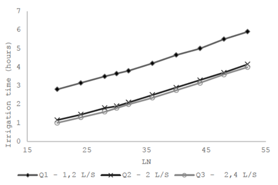
Figure 4: Optimized irrigation time with WinSRFR program, for each flow rate in different soil moisture situations
As can be seen in Figure 4, there was a difference of the order of magnitude of 100 minutes in the irrigation time of the lowest flow rate (1.2 L s-1) compared to the irrigation time of the other two flow rates evaluated (2 and 2.4 L s-1) for different LN required.
3.2 Field determinations
The irrigation evaluation dates were: 14/01/21, 15/01/22, 31/01/22, 8/04/22, 23/04/22, 30/11/22, 6/12/22 and 12/12/23. On the first three dates, on the fifth and on the last one, the three flow rates could be evaluated, while on the remaining dates only the unit flow rates of 0.2 L s-1 m-1 and 0.24 L s-1 m-1could be evaluated.
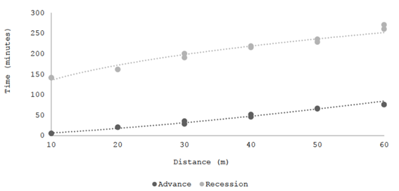
The advance and recession curves were determined for the evaluated flow rates. As an example, the result obtained for a flow rate in the evaluation of 01/31/2021 is shown. The time between the two curves corresponds to the contact time.
The inflow and outflow hydrographs measured in the evaluations were graphed. Figure 6 shows an example.
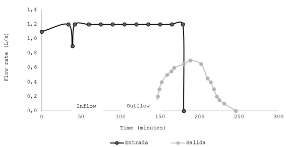
Figure 6: Example of inflow (black line) and outflow (gray line) hydrograph for unit flow rate of 0.2 L s-1 m-1 on 14/01/2021
The area under the curve of the inflow hydrograph represents the total volume of water supplied to the border, and the area under the curve of the outflow hydrograph corresponds to the total runoff volume.
3.3 Performance parameters
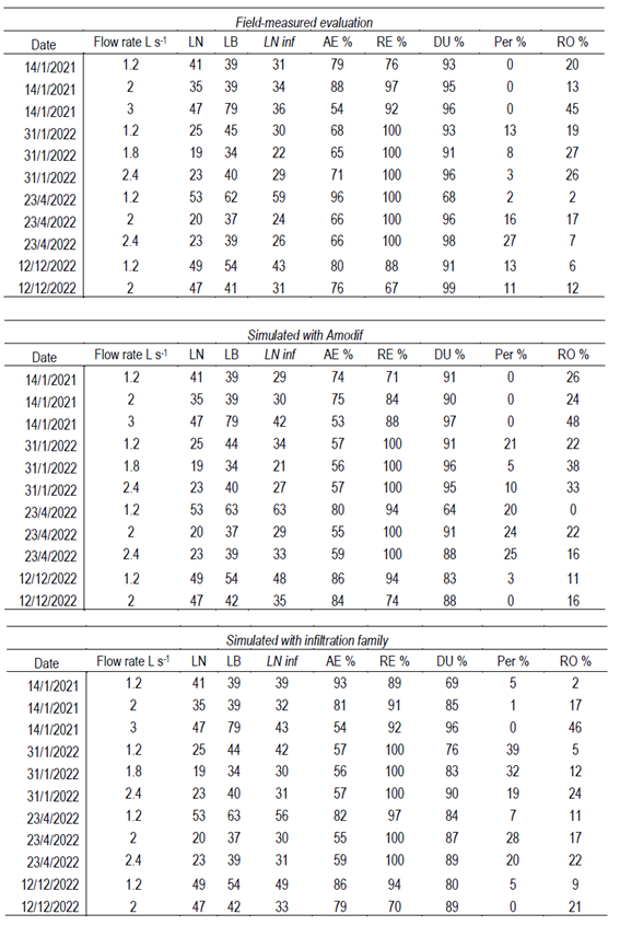
The performance parameters of the 21 irrigation events are detailed in Table 4. It presents results derived from the processed field data, parameters obtained by the infiltration rate equation, using the Amodif through the volume balance (2), and the performance parameters based on the infiltration family defined from the Ib(3).
Table 4: Measured performance parameters simulated using adjusted infiltration rate and simulated using infiltration family, for all events (total 21)
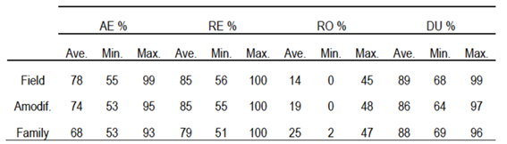
Note: Field: Field-measured evaluation. Amodif: Simulation with Amodif. Family: Simulation with infiltration family. Avg.: Average. Min.: Minimum. Max.: Maximum.
In this initial analysis (Table 4), elevated values of AE are highlighted, along with satisfactory values for DU, both in averages and minimum values. It is valuable that the minimum values recorded are aligned with the optimal expectations according to the literature for border irrigation17. Additionally, the good performance of the model in predicting parameters AE, RE and DU can be verified, both in the simulation carried out with the infiltration modified by the volume balance and in the simulation using the infiltration family, with a lower accuracy in the prediction of RO.
In the table presenting the measured values of the 11 selected events (Table 5), the lowest AE value was 65%. This high value is expected considering that the length of the borders did not exceed 64 m, but it is high regarding the steep longitudinal slopes of the borders. High AE values ± 96% were related to situations of high LN and LB relatively close to LN, indicating that the sheet of water entering the borders infiltrated almost entirely. However, since in some of these cases the LN was not completely covered to return the soil to field capacity, the value of storage efficiency did not reach 100%.
Furthermore, satisfactory and high values are evident in the DU in all evaluated cases. In this parameter, the minimum values found far exceed the 70% threshold in all three cases.
3.4 Validation of the WinSRFR model
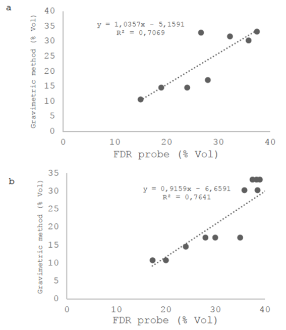
As already mentioned, the validation of the WinSRFR model was conducted using a careful selection of irrigation events. Only 11 of these events were included in the validation process, limited to those where an LN value of 54 mm or less was determined. The performance parameters corresponding to the events selected for validation are detailed in Figure 7, Figure 8, Figure 9 and Figure 10 and Table 5.
The analysis of the values obtained for the performance parameters of the 11 selected evaluations (Table 5) reveals a significant similarity in the average terms compared to the total set of evaluations (Table 4). Specifically, the average values have the following figures: LN inf = 33; AE = 74%; RE = 93%; DU = 93%; Per = 8% and RO = 18%.
It is important to highlight an improvement in the average value of RE and to point out that this improvement is attributed to the confirmation that the values of LN, LB and LN inf are lower than those obtained when considering all the evaluations together. This selective approach not only confirms the robustness of the model under specific conditions but also provides greater insight into improvements in predictions when faced with events of LN needs commonly used at the production level.
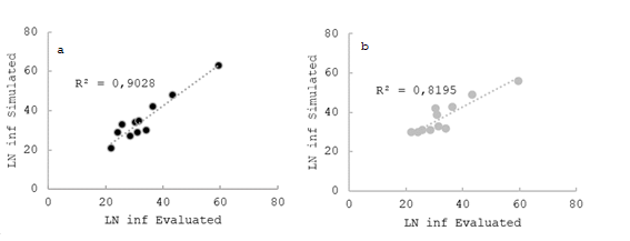
Figure 7: Net infiltration sheet (LN inf) measured in the field (evaluated) vs. predicted (simulated); a and b correspond to Simulation with Amodif and Simulation with infiltration family, respectively, in the selected evaluations
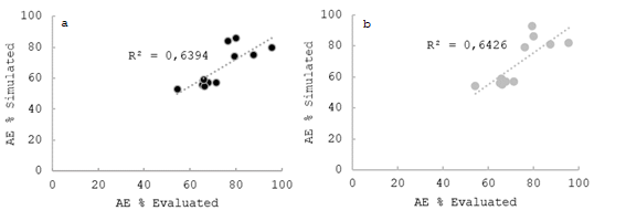
Figure 8: Application Efficiency (AE) measured in the field (evaluated) vs. predicted (simulated); a and b correspond to Simulation with Amodif and Simulation with infiltration family, respectively, in the selected evaluations

Figure 9: Storage efficiency (RE) measured in the field (evaluated) vs. predicted (simulated); a and b correspond to Simulation with Amodif and Simulation with infiltration family, respectively, in the selected evaluations
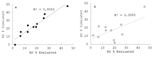
Figure 10: Runoff (RO) measured in the field (evaluated) vs. predicted (simulated); a and b correspond to Simulation with Amodif and Simulation with infiltration family, respectively, in the selected evaluations
Table 5: Measured performance parameters, simulated using adjusted infiltration rate, and simulated using infiltration family, in the evaluations selected for validation
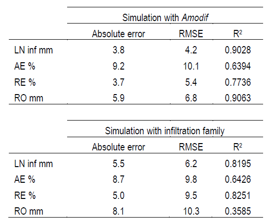
By analyzing the correlation between the evaluated data and the simulated data, it is confirmed that, in most cases, this correlation is high. When focusing on cases involving the use of Amodif, the R² values for LN inf are consistent with expectations, since this variable is influenced by the volume balance. In the same way, when observing the R² values for AE of 0.64, RE of 0.77 and RO of 0.90, it is clear that measuring the runoff at the foot and knowing precisely the value of LN inf increase the accuracy in the prediction of the values.
Simulating using the infiltration family (without considering direct runoff measurement in the field), we also noticed a similarity between predicted and observed values. The R² values for LN inf, AE, RE, and RO are 0.82, 0.64, 0.82, and 0.35, respectively. It is relevant to note that the RE values show a significantly better fit when using the infiltration family, compared to using Amodif. However, predicting runoff at the foot is less precise, as reflected in low R² values.
In terms of error analysis, it is noteworthy that these errors are minimal, both in millimeters, in the case of LN inf or RO, and in percentage terms, in the case of AE and RE. The average absolute errors for LN inf are 11 and 17%, compared to the average LN inf value obtained in the analyzed cases and for the Simulation with Amodif and Simulation with the infiltration family, respectively. In the case of AE, it is observed that the error is close to 9% in both cases, while for RE, errors range between 3 and 5%, with the situation of Simulation with Amodif and Simulation with the infiltration family, respectively. As for RO, the error is between 6 and 8 mm, taking into account that the average RO is 18%, confirming that this parameter is the most difficult to predict, with a percentage error between 33 and 44%. When analyzing the errors using the Root Mean Square Error (RMSE), a very similar trend is observed, although a higher value stands out in absolute terms for each of the performance parameters evaluated in both situations.
3.5 Sensitivity analysis
The results of the sensitivity analysis are presented below.
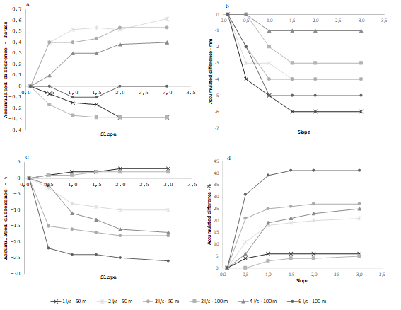
Figure 11: Accumulated difference of: a) IT (irrigation time), b) LN inf, c) AE, and d) RO at slope increments
In each quadrant of Figure 11, each line corresponds to a condition of border length and irrigation flow. These fixed conditions allow analyzing the variation of the LN inf, AE and RO parameters simulated by the model when the slope varies. It is observed that the WinSRFR model shows high sensitivity to the variations in land slope up to 1%. In the range of 1 to 2.5%, variations are minimal. After 2.5%, the sensitivity decreases even further. In this analysis, sensitivity was analyzed up to slope values between 2.5 and 3%.
The irrigation time (IT) is the sum of the advance time plus the time of opportunity for the LN to infiltrate at the foot of the border. As the slope increases, the advance time decreases, until the variation in the advance time is only affected by land roughness related to vegetation and becomes constant. Because LN inf, AE and RO are directly related to the irrigation time, the variation of these parameters as a function of the slope is no longer noticeable above the 1.5-2% slope range. Consequently, it can be stated that, in this context, the increase in slope has a marginal effect on the variation of the irrigation time, for values above 3%.
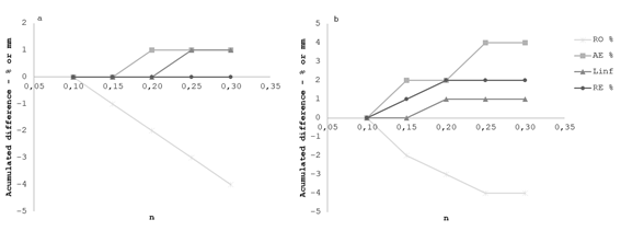
Figure 12: Accumulated difference to variations in Manning's roughness coefficient (n); a and b correspond to 2 hours and 1.3 hours of irrigation time, respectively
It is observed that the variation of the roughness coefficient (n) has a small magnitude effect on the performance parameters obtained (Figure 13 and 14). It is important to highlight that the sensitivity is higher for RO %, coinciding with the information presented by Bautista and others27.
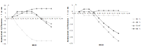
Figure 13: Accumulated difference to variations in infiltration family, at 0.1% slope; a and b correspond to 2 hours and 1.3 hours of irrigation time, respectively
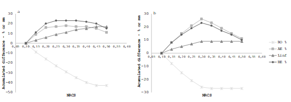
Figure 14: Accumulated difference to variations in infiltration family, at 1% slope; a and b correspond to 2 hours and 1.3 hours of irrigation time, respectively
The variation in the infiltration family demonstrates an effect on the performance parameters obtained when exploring various slope and IT conditions. The results are consistent in several aspects: large variations in RO values are observed until an infiltration family of 0.35 is reached. However, above this value, there are no significant changes in this factor. In addition, for this same situation, limited variation is observed in the term LN inf, which is the value with the least variability in the face of changes in the infiltration family.
The impact on the values of AE and RO is clear, which decreases considerably when the infiltration family exceeds 0.35. These results are consistent with the findings of Bautista and others27. It is crucial to highlight that no significant differences are observed in percentage terms between the 0.25 and 0.35 infiltration families, with these being the most predominant families in Uruguayan soils.
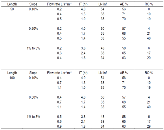
3.6 Technical recommendations for the design and management of border irrigation in pastures
Taking into account that the model shows few variations in the analyzed parameters above 2.5 and 3% slope, a table was developed that includes recommended flow rates and irrigation times for different border lengths and slopes. These results are valid for soils belonging to the same infiltration family as those used at the trial site. This guide can serve as a useful tool for irrigation technicians as a primary recommendation when defining the design and management of border irrigation in pastures for the predominant soils of Uruguay.
4. Conclusions
The results presented reveal the robustness and predictive capacity of the WinSRFR model in the evaluation of hydrological parameters and performance parameters of border irrigation for different soil and topographic conditions. The model makes a good prediction, introducing data of the infiltration family instead of direct measurements of runoff. This makes it a useful and easy-to-use tool for the design and management of border irrigation in pastures, beneficial for both technicians and producers.
Sensitivity analysis provides information on the influence of variables, such as land slope, roughness coefficient (n), and infiltration family, on model prediction. The model showed sensitivity up to slope values of 2.5 and 3%, therefore, its use should be limited to these slopes to obtain optimal hydrological parameters. Variations in the infiltration family demonstrate a significant impact on performance parameters, highlighting the need to carefully consider these variables when applying the WinSRFR model.
Error analysis and evaluation using the RMSE support the overall accuracy of the model, indicating consistency in the error trend even under varying conditions.
The development of specific management measures for different slopes and border lengths illustrates the practical applicability of the model by providing concrete recommendations to optimize irrigation management yield. It is noteworthy that the events used for the validation of the model occurred in soil conditions with reasonable moisture levels at the time of irrigation, ranging from 25 to 85% of available water depletion, representing suitable conditions for the studied soils and contributing to maintaining optimal conditions for forage production.
In summary, the validity and versatility of the WinSRFR model in evaluation, according to the analyses presented in this study, provide a solid foundation for its practical application in upcoming studies in Uruguay.

